Introduction
Heart failure (HF) is increasing in prevalence and affects an estimated 26 million people worldwide (Savarese et al. 2017). The genetics of HF and their contribution to risk factors are not well understood relative to other cardiac phenotypes, such as atrial fibrillation (Anderson et al. 2020). HF is defined by the impairment of ventricular filling or ejection of blood by the heart. There is high phenotypic variation within HF including two major manifestations: heart failure with preserved ejection fraction and heart failure with reduced ejection fraction. Perhaps partially due to this heterogeneity, there are relatively few genetic loci that have been identified to be significantly associated with HF.
One previous GWAS meta-analysis that analyzed 115,150 cases and 1,550,331 controls identified 47 risk loci for heart failure and identified 14 additional risk loci by using multivariate GWAS to integrate MRI data (Levin et al. 2022). A more recent GWAS, which stratified analyses by sex, found 2 novel risk loci in males and 1 novel risk locus in females (Yang et al. 2024). Perhaps due to the complexity of HF, many studies also use mendelian randomization with different risk factors to better understand heart failure as an outcome. Given the difficulty of identifying risk loci for HF, I thought it would be exciting to see what I discovered using the All of Us dataset, given its size and diversity of participants. My main hypotheses and predictions were:
The significantly associated variants discovered in my analysis will be concordant with previous findings.
After gene set enrichment analysis of my results, I will see significant enrichment in the oxidative phosphorylation gene set relative to other gene sets.
I may also uncover unreported variants given the size, diversity, and novelty of the All of Us dataset.
Dataset
I used the All of Us dataset which is a new biomedical dataset containing WGS and other health data on 245,400 individuals from diverse ancestries. This project was an exciting opportunity to use this dataset and may be one of the first times this dataset has been used to perform a GWAS on HF.
Given the size of the dataset, while I was initially interested in using the full dataset, it became clear to me that it would be difficult and out of the scope of the project to densify the VDS, which contains all variants in the WGS dataset, into a usable format for my analyses. Therefore, I opted to use the Allele Count/Allele Frequency (ACAF) threshold callset. The ACAF callset includes all variants with population-specific allele frequency > 1% or population specific allele count > 100 within each ancestry subpopulation. While this dataset excludes rare variants the total number of SNPS is 99.25 million compared with the 1 billion total SNPs in the full dataset. Despite this potential limitation, this was still an opportunity to perform a GWAS on a unique dataset and compare my results to previous findings.
Given that I am a beginner with these methods and have never worked with such a large dataset before, I needed to take some steps to improve the efficiency of the analysis. I quickly learned that sub-setting data to test all of my analyses before running them on the full dataset was necessary. As such I used plink to subset 1000 individuals and ran my full analysis only with this subset for chromosome 22 before running it on the full dataset. During my analysis with the full dataset, I also requested 96 cores and 100 GB of RAM and used multithreaded options in Plink2 and REGENIE whenever possible. Even so, each analysis step (QC, GWAS, and enrichment analysis) ran on the scale of hours to days, which I am not accustomed to when working with smaller datasets. Additionally, some tools, such as MAGMA, do not have multithreaded options and thus took long periods of time to run. One last approach I had to take was analyzing the data split by chromosomes instead of as a full dataset because given the size of the dataset, the analysis tools would not perform on the full dataset. While this approach was efficient, it poses a potential limitation based on how REGENIE works, which I discuss more below. Even though the ACAF callset probably was not the ideal dataset and my methods could be refined, I am glad that I now have experience working with a large dataset like All of Us.
Computing Environment
One major challenge and learning opportunity for this project was working in the All of Us researcher workbench. The All of Us researcher workbench is a cloud computing environment that allows researchers to analyze data in an environment that is compliant with security standards for sensitive health data. There were some difficulties with this environment in that it required that I download a lot of my own software, including REGENIE, BGEN, and MAGMA (Plink is preinstalled). Additionally, many packages are easily downloadable using conda but reserachers are not able to create conda environments in All of Us. Another issue is that the environment can take a long time (10–15 min) to activate and sometimes crashes or is unresponsive. I also learned about working in a cloud environment and storing and retrieving data from google buckets, which was necessary for data access and management in the All of Us researcher workbench. I appreciate many features of the researcher workbench and it is not extremely difficult to use once you get used to it.
Defining the Heart Failure Phenotype
One initial challenge that came up in my analysis was defining the HF phenotype. While the lab I joined this year, the iCaMP lab, focuses on cardiac problems like HF, I have limited understanding of HF. I did not have a chance to confer with one of the experts in my lab so I ended up just casting a wide net and choosing all of the ICD10 codes associated with HF in any way. After later discussion with Seung Hoan Choi, he pointed out to me that HF is a heterogeneous phenotype and likely I would have more significant associations if I defined the phenotype less broadly and focused on one specific type of heart failure, such as systolic heart failure. Modifying the phenotype definition could be a future direction of this analysis.
Quality Control
One benefit of using the ACAF callset instead of the full dataset is that the All of Us consortium performed quality control on the dataset before they made it available. They removed variants that did not pass preset filters for heterozygosity and variant call quality. I used the Plink formatted files from ACAF sharded by chromosome. Another learning opportunity would have been to use the BGEN files, which are a popular file format for GWAS analyses.
Even though quality control had been performed on the ACAF, I wanted to set my own thresholds and perform quality control before my analysis in case my thresholds were more stringent. I filtered data based on missingness of variants, Hardy-Weinberg equilibrium of variants, minor allele frequency, heterozygosity of individuals, and missingness of individuals. For each chromosome I filtered out variants with missingness > 0.05, Hardy-Weinberg test p-values < 1E-6, and minor allele frequency < 0.01. I also calculated individual missingness for each chromosome, performed LD pruning of variants with a 500 kb window and an R2 threshold of 0.1, and used pruned variants to calculate heterozygosity. After analyzing all chromosomes individually, I averaged individual missingness and heterozygosity across chromosome and analyzed the distributions to determine outlier exclusion thresholds (Figures 1 & 2).
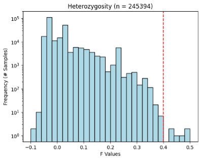
Figure 1. Heterozygosity of ACAF dataset. Red line shows QC exclusion threshold.
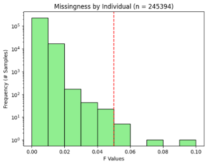
Figure 2. Missingness by individual in ACAF dataset. Red line shows QC exclusion threshold.
REGENIE GWAS
My dataset was unbalanced as it contained 232,996 controls and only 12,383 HF cases. For this reason, I used the REGENIE method for my GWAS which is designed for unbalanced phenotypes (Mbatchou et al. 2021). REGENIE involves first reducing dimensionality of data by sub-setting SNPs into blocks and for each block calculates ridge regressions, which is a method for multivariate regression when predictors are not independent. The ridge regression accounts for LD within blocks but not between blocks. I chose a block size of 100 SNPs since I assumed that my SNPs would be less densely distributed across positions since I was only using common variants. Since the ridge regression does not account for LD between blocks, I am now thinking that perhaps testing my analysis with larger and fewer blocks (e.g. block size = 1000) may better account for LD – this would be an interesting comparison. However, the developers of REGENIE suggest that block size is more important for computational efficiency and has a minimal impact on outcome of variant-phenotype associations.
The next step of REGENIE is to combine the ridge regression predictors into a single predictor with a second ridge regression that builds a genome scale regression model. Genetic prediction ignoring chromosome is also calculated using the leave one chromosome out (LOCO) method, which generates covariates to account for relationships with chromosomal location among variants. I looked into this because I had to split my inputs by chromosome in order to get them to run and I think that this may be a limitation of my approach, because the LOCO method does not provide additional information if you are only running the analysis on a single chromosome as far as I can understand. The last step of REGENIE uses the model, which is validated with k-fold leave-one-out-cross-validation, to determine the association between phenotypes and each SNP. So, in my analysis, I really built a whole chromosome model for each chromosome, not a whole genome model and the information about genomic location for each SNP was functionally not included in the model. This would be something to improve upon for another iteration of this study.
I used the following linear model in my GWAS, with the PCs generated by the All of Us consortium explaining the top 5 highest percent variance explained used as covariates to adjust for population structure:
Logit(pi) = B0 + B1(Additively coded allele) + B2(sex) + B3(age) + … +Bi(PCj)
GWAS Results
My GWAS results did not show any variants that reached the genome-wide significance threshold but did show some variants that are approaching significance (Table 1, Figure 3). The QQplot shows that the models perform somewhat well with lambda near to 1, but that the model consistently underestimates p-value (Figure 4). This result suggests that the model needs to be improved.
I also searched the full set of SNPs I used in my GWAS post-QC for the 47 variants identified by Levin et. al 2022 and was unable to find any of them in my dataset, meaning that they were possibly filtered out with QC, or more likely not present to begin with in the ACAF callset. Additionally, I searched the top 5 most significant variants in the Open Targets Genetics Database and found that chr12:129603762:A:G, chr3:88052189:T:C, and chr2:227388735:C:G were previously found to have non-significant associations with cardiovascular disease and musculoskeletal or connective tissue disease. Interestingly I could not find chr1:88837391:CAAAAAAA:C in the Open Targets database, suggesting it may be a relatively rare or new variant discovered in All of Us. There is more analysis I could do here with respect to identifying individual variants of interest, such as fine-mapping.
There are a variety of improvements or modifications I could make to my GWAS including running step1 of Regenie on the full dataset instead of splitting by chromosome, including more than 5 PCs as covariates, more specifically defining the HF phenotype, and setting more stringent QC thresholds. Another iteration of this analysis that incorporates some of these improvements may also build confidence in these initial results.
Table 1. GWAS Initial Results: Ranked Top 5 Lowest P-value SNPS. None reach genome wide significance threshold (5E-8).
| Rank | SNP ID | Genome Location | pvalue | OR |
|---|---|---|---|---|
| 1 | chr12:129603762:A:G | TMEM132D (Intron) | 9.2E-7 | 1.09 |
| 2 | chr3:88052189:T:C | CGGBP1 (3’ UTR) | 1.4E-6 | 1.32 |
| 3 | chr2:227388735:C:G | H3K27Ac Mark (Regulatory) | 1.5E-6 | 0.92 |
| 4 | chr5:93501319:TTTG:T | NR2F1 antisense RNA (Intron) | 1.6E-6 | 0.93 |
| 5 | chr1:88837391:CAAAAAAA:C | H3K27Ac Mark | 1.9E-6 | 0.80 |

Figure 3. Manhattan plot of GWAS results showing distribution of regression p-values across genomic coordinates.
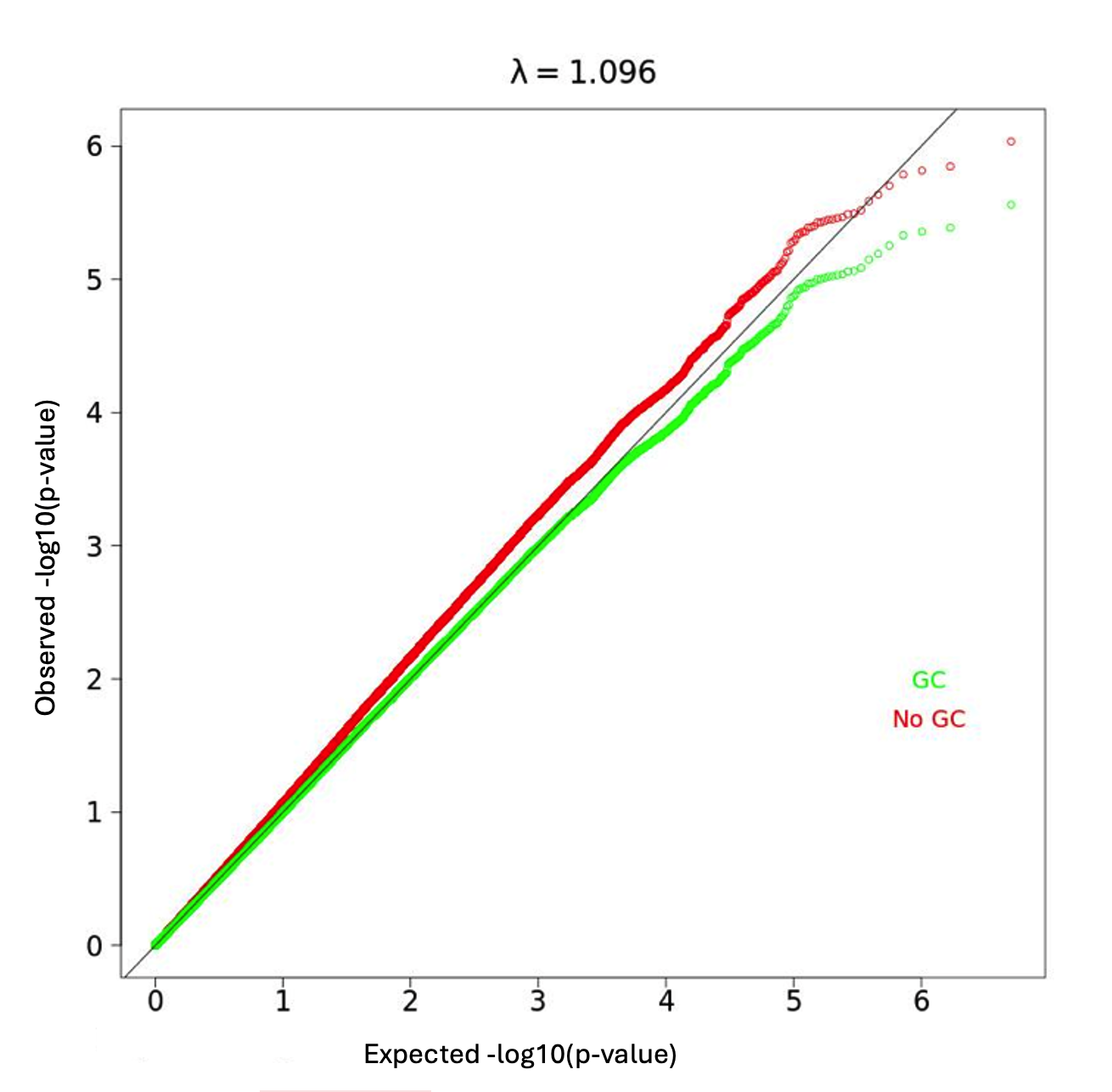
Figure 4. QQplot of all variants. λ = 1.096.
Lastly, I used MAGMA to perform a gene enrichment analysis and a gene set enrichment analysis using the hallmark human gene set from the Molecular Signatures Database. The gene enrichment analysis showed that the genes with the largest amounts of SNPs still had relatively high p-values (minimum p-value = 1.4E4, Bonferroni-adjusted p-value threshold = 2E-6). The gene set enrichment did show some significant results (Table 2), most notably related to mesenchymal transition and apical surface. Mesenchymal transition is related to both cancer metastasis and wound healing, however I do not know how much relevance either of these processes have to HF. Notably, oxidative phosphorylation genes were not significantly enriched (p = 0.80655), which does not support my initial hypothesis that there would be more variants associated with HF in oxidative phosphorylation genes. It would be interesting to do further gene set enrichment analyses on other gene sets with this GWAS dataset in the future.
Table 2. Top 3 significantly enriched gene sets of 50 gene sets in Molecular Signatures Hallmark gene sets database.
| Name | Beta | pvalue | # Genes |
|---|---|---|---|
| EPITHELIAL_MESENCHYMAL_TRANSITION | 0.15754 | 0.0073483 | 192 |
| APICAL_SURFACE | 0.34037 | 0.0081267 | 41 |
| SPERMATOGENESIS | 0.11094 | 0.063192 | 129 |
To conclude, I am glad that I had the opportunity to use the All of Us dataset for this project. My hypothesis that I would be able to replicate results from previous studies was not supported by my results, likely because I used the ACAF callset and potentially also as a result of some my methods. I also did not see enrichment of oxidative phosphorylation genes in my called variants as I had predicted and did not uncover any new genome-wide significant variants in my analysis. While my study had some major limitations based on the data and potentially the analysis methods, it gave me exposure to the process of performing a GWAS on a large dataset and the many challenges that need to be addressed while doing so.
Source Code
attach github link
References
Andersen, Julie H., Laura Andreasen, and Morten S. Olesen. "Atrial fibrillation—a complex polygenetic disease." European Journal of Human Genetics 29.7 (2021): 1051-1060.
Mbatchou, Joelle, et al. "Computationally efficient whole-genome regression for quantitative and binary traits." Nature genetics 53.7 (2021): 1097-1103.
Savarese, Gianluigi, and Lars H. Lund. "Global public health burden of heart failure." Cardiac failure review 3.1 (2017): 7.
Yang, Qianqian, et al. "Sex-stratified genome-wide association and transcriptome-wide Mendelian randomization studies reveal drug targets of heart failure." Cell Reports Medicine (2024).